Environmental Dose Rate Calculation - DRAC vs RCarb
by Sebastian Kreutzer (March 3, 2021)

Creative Commons
Attribution-NonCommercial-NoDerivatives 4.0
International License
The calculation of the environmental dose rates (\(\dot{D}\)) is crucial for luminescence-dating studies. Right or wrong matters because it makes the other 50% of your luminescence age equation. Quick reminder:
\[ Age~ {[ka]} = \frac{Equivalent~dose~[Gy]}{Dose~rate~[Gy/ka]} \] Today, I received an exciting message asking me why the \(\dot{D}\) calculated with RCarb (Kreutzer et al. 2019) differs from the one calculated with DRAC (Durcan, King, and Duller 2015). It appeared to be easy, but it turned out to be a little bit of a tricky task. I assume that others may run into a similar problem. They might then start questioning the correctness of the results returned by DRAC or RCarb or even both. I can put the minds at ease: the results are comparable (as expected); if the calculation parameters were set correctly. This is the tricky part, and it might be of interest to others, so I decided to put it into writing. What you will find below is not a tutorial but a showcase of how to test different tools.
Background (skip to cut to the chase)
Stop! What were DRAC and RCarb again? Both are software tools to calculate environmental dose rates needed to calculate luminescence ages. DRAC is an online tool initially developed by my colleagues (Durcan, King, and Duller 2015) here at Aberystwyth University, and the service is still hosted on the servers here. How does it work? The user provides all information, e.g., on the radionuclide concentrations as CSV-file uploads the data, and a PHP script on the server calculates dose rates and even luminescence ages from the imported data. Best guess: DRAC is today the perhaps most often used software tool in the luminescence-dating community. At least it should because it couldn’t be easier to calculate a luminescence age.
Contrary, RCarb is a dose-rate modelling tool for carbonate-rich samples initially developed by Nathan and Mauz (2008) and further advanced by Mauz and Hoffmann (2014). You don’t need this very often, but you are happy to have it if you do. In 2018 I had to deal with carbonate-rich samples and tried Carb, the Matlab version of RCarb. I realised quickly that I could not use this tool on my samples because it was written in Matlab and I did not have one of those precious licences. More importantly, even after I tried a test version of Matlab, it did not work because some of the code was already too old to run on recent versions of Matlab. Long story short, supported by the original authors of Carb, I transferred the code into an R package, which I named RCarb.
So, while DRAC is a tool you would use every-day, RCarb is something you undust every once and while or never. Nevertheless, besides a new age accounting for the replacement of water by carbonate in sediment pores, RCarb also returns an age and a dose rate you would get when there was no carbonate. This number should be somewhat comparable to what DRAC returns, or something is wrong.
Compring DRAC and RCarb
The easiest way to compare calculation results is to use the example dataset shipped with RCarb. This dataset was re-checked multiple times, and it should be ok. For cross-checking the results with DRAC, we could use the online service or, easier for our purpose, the R package Luminescence. The latter comes with an API to interface DRAC with R. We will go for this.
The first step is to load the packages and datasets we need:
## load pacakges
library(Luminescence)
library(RCarb)

## load example dataset from RCarb
data("Example_Data", envir = environment())
No dataset is perfect. We have to remove one dataset with an equivalent dose of 0 (here row number 23).
Example_Data <- Example_Data[-23, ]Because the modelling does a little bit more than just calculating numbers, we should tweak our dataset by setting the final water content to the initial water content, and the carbonate concentration is set to 0.
Example_Data$WCI <- Example_Data$WCF
Example_Data$WCI_X <- Example_Data$WCF_X <- 2
Example_Data$CC <- 0
Example_Data$CC_X <- 0
Now we create a template object to interact with the DRAC API in Luminescence.
input <- template_DRAC(preset = "DRAC-example_quartz", nrow = nrow(Example_Data))This was the easy part. In the next step, we have to ensure that the results can be comparable by setting similar parameters.
- The dose-rate conversion factors should be the same in DRAC and RCARB. I opt for the one by Adamiec and Aitken (1998).
- RCarb only supports the \(\beta\)-dose attenuation factors by Mejdahl (1979), so we have to select this option also for DRAC.
- RCarb does not know about etching depths and assumes that the outer \(\alpha\)-dose rate effected rim of a grain was already removed.
Putting this into R code, it will look as follows:
input$`Conversion factors` <- rep("AdamiecAitken1998", nrow(Example_Data))
input$`beta-Grain size attenuation ` <- rep("Mejdahl1979", nrow(Example_Data))
input$`beta-Etch depth attenuation factor` <- rep("X",nrow(Example_Data))
input$`Etch depth min (microns)` <- rep(0, nrow(Example_Data))
input$`Etch depth max (microns)` <- rep(0, nrow(Example_Data))
The rest is fairly straight forward because we just have to use the values
from the example dataset and feed them into input.
input$`External U (ppm)` <- Example_Data$U
input$`errExternal U (ppm)` <- Example_Data$U_X
input$`External Th (ppm)` <- Example_Data$T
input$`errExternal Th (ppm)` <- Example_Data$T_X
input$`External K (%)` <- Example_Data$K
input$`errExternal K (%)` <- Example_Data$K_X
input$`Grain size min (microns)` <- Example_Data$DIAM - Example_Data$DIAM_X
input$`Grain size max (microns)` <- Example_Data$DIAM + Example_Data$DIAM_X
input$`Water content ((wet weight - dry weight)/dry weight) %` <- Example_Data$WCI
input$`errWater content %` <- Example_Data$WCI_X
input$`User cosmicdoserate (Gy.ka-1)` <- Example_Data$COSMIC
input$`errUser cosmicdoserate (Gy.ka-1)` <- Example_Data$COSMIC_X
input$`a-value` <- input$`erra-value` <- rep(0, nrow(Example_Data))
input$`De (Gy)` <- Example_Data$DE
input$`errDe (Gy)` <- Example_Data$DE_X
The last step calls DRAC and RCarb to run the calculations.
## run DRAC calculation
output_DRAC <- use_DRAC(input, print_references = FALSE, verbose = FALSE)

# run RCarb calculation
output_RCarb <- model_DoseRate(
  data = Example_Data,
  n.MC = 2,
  plot = FALSE,
  verbose = FALSE,
  txtProgressBar = FALSE
)
Are the results comparable? Let’s see what we got in terms of \(\dot{D}\).
## set plot
plot(NA,NA,
     xlim = c(0, 1.8),
     ylim = c(0, 1.8),
     xlab = "DRAC dose rate [Gy/ka]",
     ylab = "RCarb dose rate [Gy/ka]",
     main = "DR DRAC vs RCarb"
)

## add control lines
abline(a = c(0,1))
abline(a = c(0,1.1), lty = 2)
abline(a = c(0,.9), lty = 2)
text(
  x = c(1.6, 1.4, 1.65),
  y = c(1.6, 1.6, 1.4),
  labels = c("1:1", "+10 %", "-10%")
)

## add data points
points(
  x = output_DRAC$DRAC$highlights$`Environmental Dose Rate (Gy.ka-1)`,
  y = output_RCarb$DR_CONV
)

## add error bars
segments(
  x0 = output_DRAC$DRAC$highlights$`Environmental Dose Rate (Gy.ka-1)` -
    output_DRAC$DRAC$highlights$`errEnvironmental Dose Rate (Gy.ka-1)`,
  x1 = output_DRAC$DRAC$highlights$`Environmental Dose Rate (Gy.ka-1)` +
    output_DRAC$DRAC$highlights$`errEnvironmental Dose Rate (Gy.ka-1)`,
  y0 = output_RCarb$DR_CONV,
  y1 = output_RCarb$DR_CONV)

segments(
  y0 = output_RCarb$DR_CONV + output_RCarb$DR_CONV_X,
  y1 = output_RCarb$DR_CONV - output_RCarb$DR_CONV_X,
  x0 = output_DRAC$DRAC$highlights$`Environmental Dose Rate (Gy.ka-1)`,
  x1 = output_DRAC$DRAC$highlights$`Environmental Dose Rate (Gy.ka-1)`)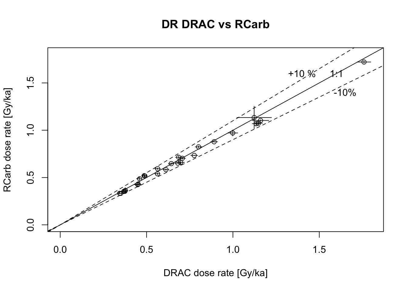
Admittedly, the results do not sit perfectly on the 1:1 line. However, there are no systematic effects, and both tools end up with highly comparable \(\dot{D}\)s.
Where are the minor differences coming from? The interpolation and the rounding of the numbers is not entirely identical.
Should I use DRAC or RCarb? It depends on your samples and their origin. Suppose your samples originate from an environment where the replacement of water by carbonate does not play a role; you should stick to DRAC.