2.1 Option 1 - Huntley and Lamothe (2001)

In 2001 Huntley and Lamothe proposed a method to correct for fading in feldspars. The method is based on the assumption that tunnelling will occur for more proximal electron-hole pairs first, with more distal electron-hole pairs being involved in the tunnelling process as time progresses. Thus, the number of trapped electrons decrease with time. It follows that the measured luminescence intensity (I) decreases linearly with the logarithm of time t, following:

\[ I = I_c [1-k * ln(\frac{t}{t_c})] \]

Here \(I_c\) is the luminescence intensity at the arbitrary time \(t_c\), and \(k\) is a constant, which describes the fractional decrease in intensity.

Visocekas (1985) proposed to express the the loss of luminescence intensity with \(ln(t)\) as percent decrease during a factor of 10 in time, for which \(g\) is used. The relationship between \(g\) and \(k\) is:

\[ g = 100*k*ln(10) \]

The unit for \(g\) is \(\%/decade\), with a decade corresponding to the factor of 10 in time since the start of the irradiation. Following this we can transform the equation describing the loss of luminescence intensity with time according to:

\[ I = I_c[1-\frac{g}{100}log_{100}(\frac{t}{t_c})] \]

Huntley and Lamothe (2001) call for caution when using this equation for fading correction over geological time scales, as errors might be introduced either over too short or too long measurement time scales. Huntley and Lamothe (2001) tested and adapted their equation for the use on geological time scales, which results in the following equation:

\[ I_f = I_0(1-k[ln(\frac{T}{t_c})-1]) \]

Here \(I_f\) is the luminescence intensity which has been affected by fading, \(I_0\) the intensity if it would not have been affected by fading, \(k\) is a constant, \(T\) is the time over which the irradiation occurred (in nature this would be the luminescence age). For simplicity reasons \(t_c\) is the time between the laboratory irradiation and the luminescence measurement.

If one now wishes to correct their luminescence age for fading, then this can be done following:

\[ \frac{T_f}{T} = \frac{D_{ef}}{D_e} = \frac{I_f}{I_0} = 1 - k[ln(\frac{T}{t_c})-1] \]

where the intensity \(I\), the equivalent dose \(D_e\) and the age \(T\) are all proportional. \(T_f\), \(D_{ef}\) and \(I_f\) are values affected by fading, \(T\), \(D_e\) and \(I_0\) are the values for age, equivalent dose and luminescence intensity, if they were not affected by fading. \(T\) is the true age and \(t_c\) is the time between the laboratory irradiation and luminescence measurement.

The function calc_FadingCorr() uses this correction approach to correct an age.faded with a given \(g_{value}\). A value for \(t_c\) needs to be inserted, which depends on the measurement protocol, irradiation time and instrument used to perform the fading test. The value can be retrieved from the measurement sequence results (i.e. on a Risø reader the generated .binx file lists this as \(time since irradiation\), which can be viewed in \(Analyst\).) A further \(Tc.g_{value}\) is needed, which corresponds to the time used for normalisation, usually two days, which corresponds to 172,800\(\,\)s.

The following piece of code is an example for the use of the calc_FadingCorr() function, where age.faded (and the uncertainty) is given in kilo years. The g-value needs to be provided. This can either be a g-value calculated in another programme (e.g. Analyst) or a g-value obtained by analysing fading data using the analyse_FadingMeasurement() function in the 'Luminescence' package. An example on how this function can be used is given in the next section.

library(Luminescence)
calc_FadingCorr(
   age.faded = c(13.7,1.6),
   g_value = c(3.2, 0.7),
   tc = 718,
   tc.g_value = 172800,
   n.MC = 500)

## 
## 
## [calc_FadingCorr()]
## 
##  >> Fading correction according to Huntley & Lamothe (2001)
##  >> g-value re-calculated for the given tc
## 
##  .. used g-value:	2.973 ± 0.689 %/decade
##  .. used tc:		2.275e-08 ka
##  .. used kappa:		0.0129 ± 0.003
##  ----------------------------------------------
##  seed: 			NA
##  n.MC: 			500
##  observations: 		500
##  ----------------------------------------------
##  Age (faded):		13.7 ka ± 1.6 ka
##  Age (corr.):		18.3128 ka ± 2.6164 ka
##  ----------------------------------------------

## 
##  [RLum.Results-class]
## 	 originator: calc_FadingCorr()
## 	 data: 2
##  	 .. $age.corr : data.frame
## 	 .. $age.corr.MC : numeric
## 	 additional info elements:  1

2.2 Option 2 - Huntley (2006)

The fading correction method by Huntley and Lamothe (2001) uses a logarithmic approximation for the signal loss due to fading. However, this approximation cannot be used for very short or very long decay times. As an alternative, Huntley (2006) proposed a fading correction method, describing the quantum mechanical tunnelling process, the mechanism behind anomalous fading, as a function of of the lifetime of the tunnelling decay \(\tau\), the distribution of distances (\(r\)) between electron trapping centres and recombination centres and the density of recombination centres \(\rho\)’. Kars et al. (2008) used the theoretical considerations made by Huntley (2006) and developed a model which simulates natural fading in feldspars. The model by Kars et al. (2008) enables the reconstruction of an un-faded dose response curve, as well as the construction of the dose-response curve at dose rates in found in nature. Furthermore the model can predict field saturation levels and fading rates for the IRSL signals in field saturation.

Details regarding the model from Huntley (2006) and their applications are given in Kars et al. (2008). Here we would like to highlight some equations which are more relevant for the understanding of the natural fading simulation model by Kars et al. (2008).

Huntley (2006) explains that fading and the amount of trapped electrons remaining after delay time \(t\) is dependent on the density of recombination centres (\(\rho\)’) in the crystal, where \(n\) is the trapped electron density remaining after time \(t\) and \(n_i\) the initial trapped electron population. \(s\) represents the attempt-to-escape frequency, which is assumed to be \(3\times10^{15}\) s^-1 (Huntley, 2006).

\[ \frac{n}{n_i} = exp(-\rho'[ln(st)]^3) \]

Huntley (2006) substitutes \(st\) by \(1.8st\). Since the portion of electrons still trapped after delay time \(t\) is dependent on the \(\rho\)’, and the IRSL signal intensity is the result of the number of trapped charges recombining, Kars et al. (2008) rewrite the equation to

\[ IRSL_{faded} = IRSL_{initial} * exp(-\rho'[ln(1.8st)]^3) \]

Besides calculating the initial IRSL signal by using the above given relationship, Kars et al. (2008) also adapt the model from Huntley (2006) to calculate the dose response curve if the IRSL signal measured would not have faded using the equation given above.

The 'Luminescence' package enables the use of the natural fading simulation model by Kars et al. (2008) by using the function calc_Huntley2006(). The package and function provide an example data set for performed fading measurements and for equivalent dose measurements. These example data sets can be called by running the following:

library(Luminescence)

## Load example data (sample UNIL/NB123, see ?ExampleData.Fading)
data("ExampleData.Fading", envir = environment())

## (1) Set all relevant parameters
# a. fading measurement data (IR50)
fading_data <- ExampleData.Fading$fading.data$IR50

# b. Dose response curve data
data <- ExampleData.Fading$equivalentDose.data$IR50

The example data $ExampleData.Fading contains a list of two, one list containing the fading data and one containing the equivalent dose data. The fading data consists of a list of four data.frame with \(\frac{T_x}{T_x}\) values and their uncertainties and the time since irradiation for each \(\frac{T_x}{T_x}\) value measured. The equivalent dose data contains a list of four data.frame with doses in s and measured \(\frac{T_x}{T_x}\) values for the dose response curves measured. For optimal performance of the model and to obtain the most accurate results, it is important that both, the fading and the dose response curve data, are well constrained.

For the model to run, some further information is needed. This includes the environmental dose rate ddot, as well as the dose rate of the beta source used for the measurements readerDdot.

## (2) Define required function parameters
ddot <- c(7.00, 0.004)
readerDdot <- c(0.134, 0.0067)

Furthermore an estimate of \(\rho\)’ is needed to run the calc_Huntley2006() function. This value can be extracted by using the analyse_FadingMeasurement() function in the 'Luminescence' package.

# Analyse fading measurement and get an estimate of rho'.
# Note that the RLum.Results object can be directly used for further processing.
# The number of MC runs is reduced for this example
rhop <- analyse_FadingMeasurement(fading_data, plot = TRUE, verbose = FALSE, n.MC = 10)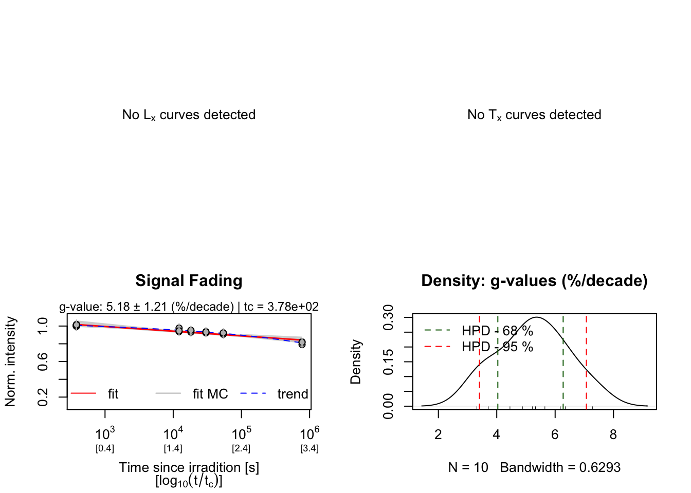

Now we have obtained all parameters required to run the actual model:

## (3) Apply the Kars et al. (2008) model to the data
kars <- calc_Huntley2006(
 data = data,
 rhop = rhop,
 ddot = ddot,
 readerDdot = readerDdot,
 n.MC = 25,
 fit.method = "EXP")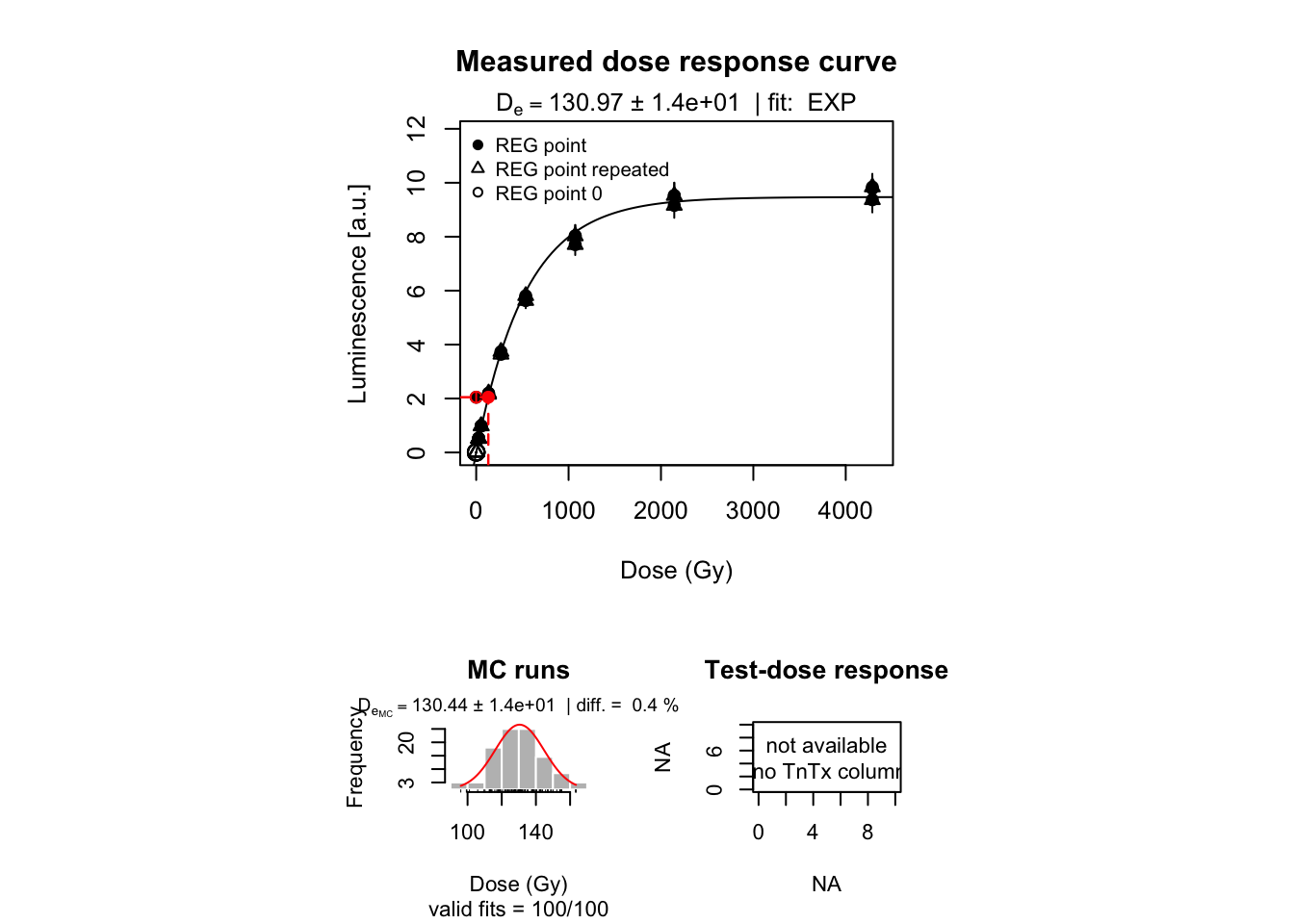

## 
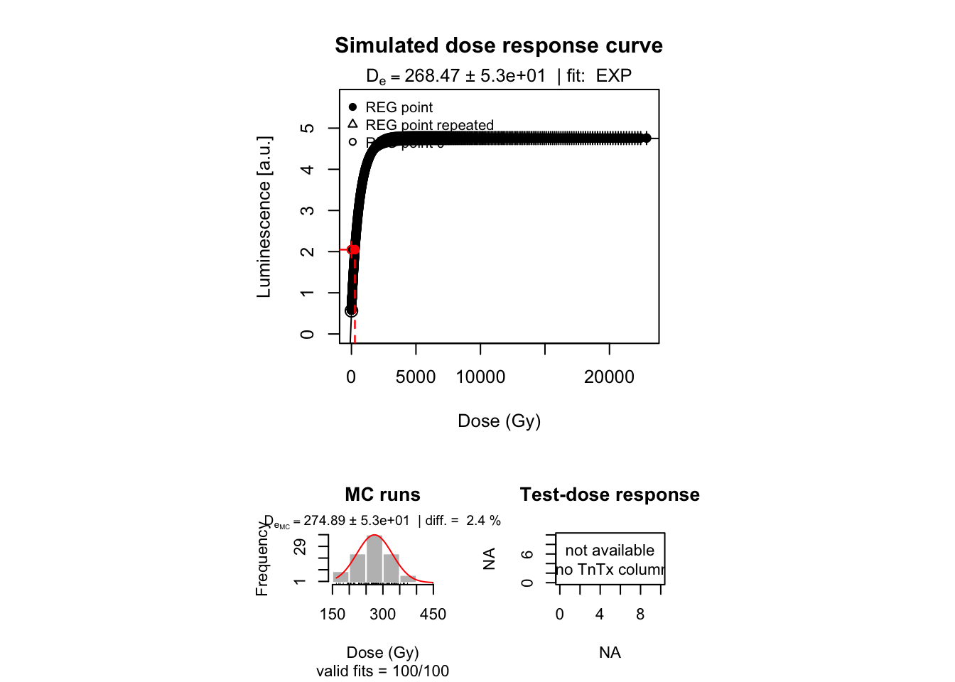
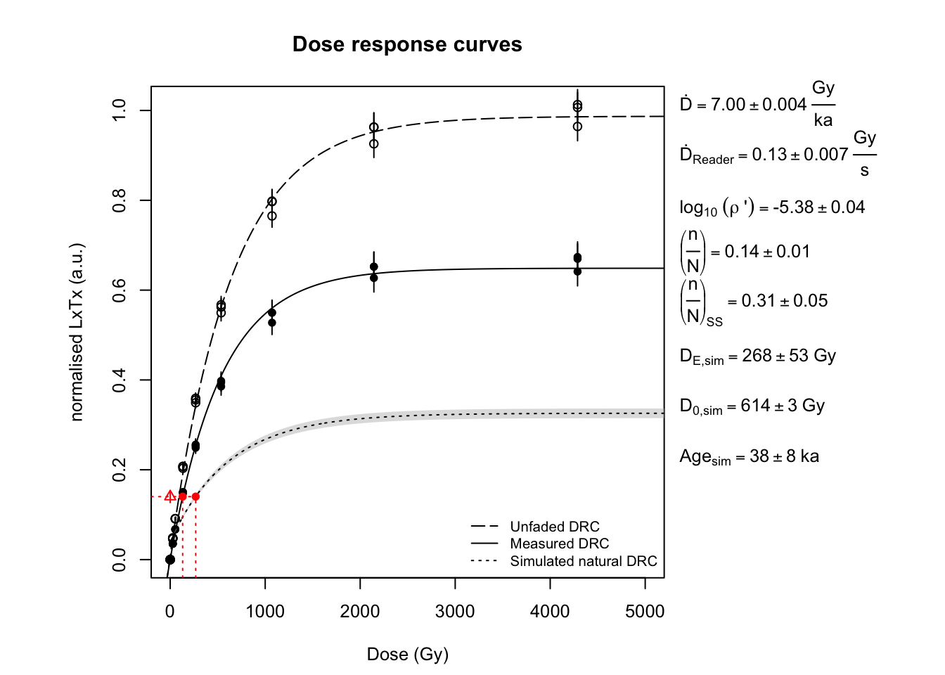
## [calc_Huntley2006()]
## 
##  -------------------------------
##  (n/N) [-]:	 0.14 ± 0.01
##  (n/N)_SS [-]:	 0.31 ± 0.05
## 
##  ---------- Measured -----------
##  DE [Gy]:	 130.97 ± 14.33
##  D0 [Gy]:	 539.01 ± 19.34
##  Age [ka]:	 18.71 ± 2.25
## 
##  ---------- Un-faded -----------
##  D0 [Gy]:	 642.72 ± 13.46
## 
##  ---------- Simulated ----------
##  DE [Gy]:	 268.47 ± 52.66
##  D0 [Gy]:	 613.98 ± 3.37
##  Age [ka]:	 38.35 ± 7.76
##  Age @2D0 [ka]:	 175.42 ± 8.82
##  -------------------------------

The output of running the model consists of a series of figures as well as an RLum.Results object. The RLum.Results object generated (here saved as kars) returns a data.frame with the results of the Kars et al. (2008) model, as well as data.frame containing the input data. Furthermore, the unfaded natural \(L_n\) value and its uncertainty is given. \(\frac{L_x}{T_x}\) values for all dose response curves generated are given, as well as details on the fits. The console also gives out the most important results, including the saturation level \(\frac{n}{N}\), the measured and simulated De, D0, and Age.

Further details to the function calc_Huntley2006() are given in the help section of the 'Luminescence' package.

We have now looked in detail at the application of the model by Huntley (2006) in the version presented by Kars et al. (2008). Whilst Kars et al. (2008) use an exponential fit to describe their dose response curve, it is also possible to use a general order kinetics (GOK) fit following Guralnik et al. (2015). If this is desired the code can be changed to:

## (3) Apply model to the data using the GOK fit according to Guralnik et al. (2015)
guralnik <- calc_Huntley2006(
 data = data,
 rhop = rhop,
 ddot = ddot,
 readerDdot = readerDdot,
 n.MC = 25,
 fit.method = "GOK")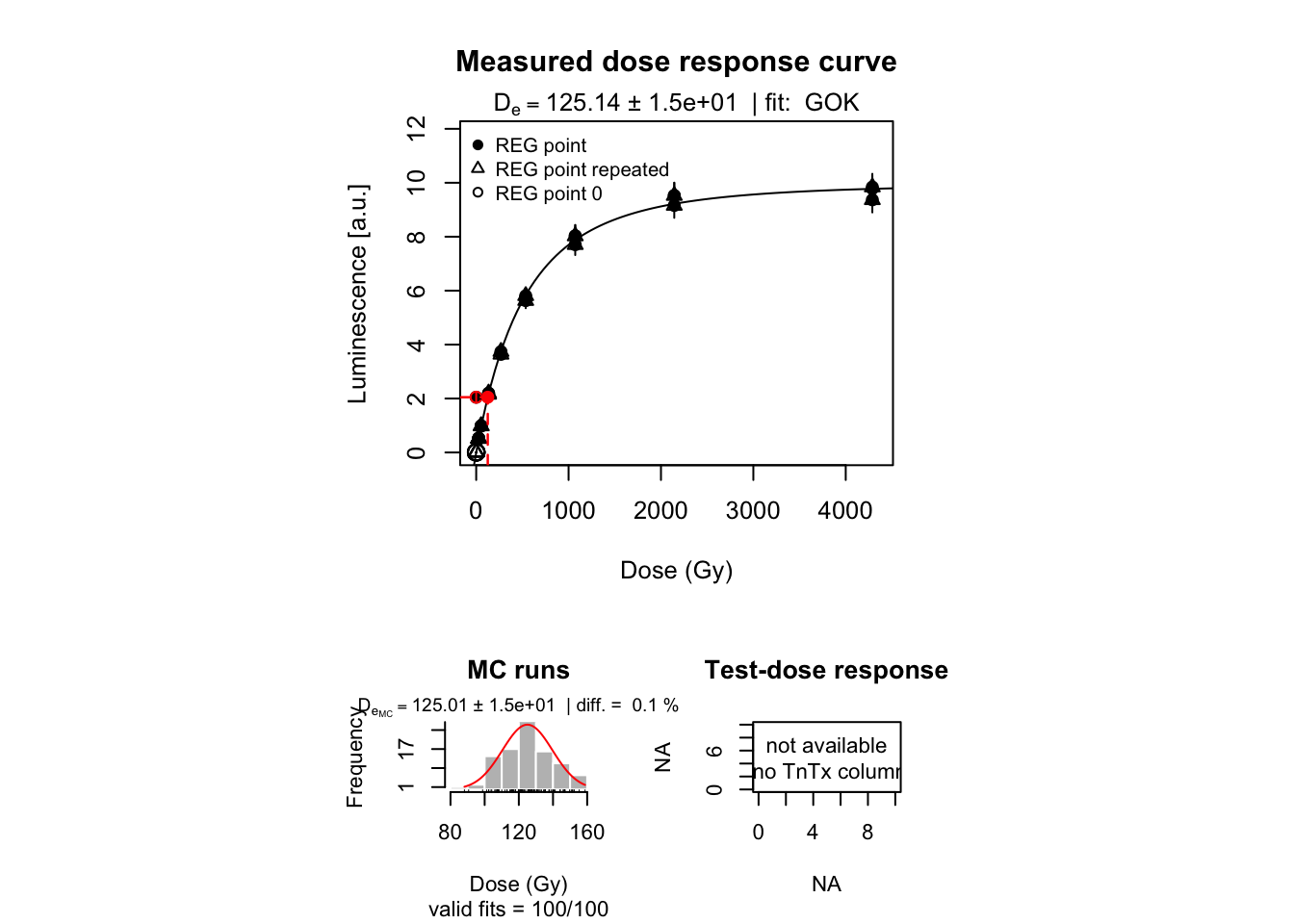

## 
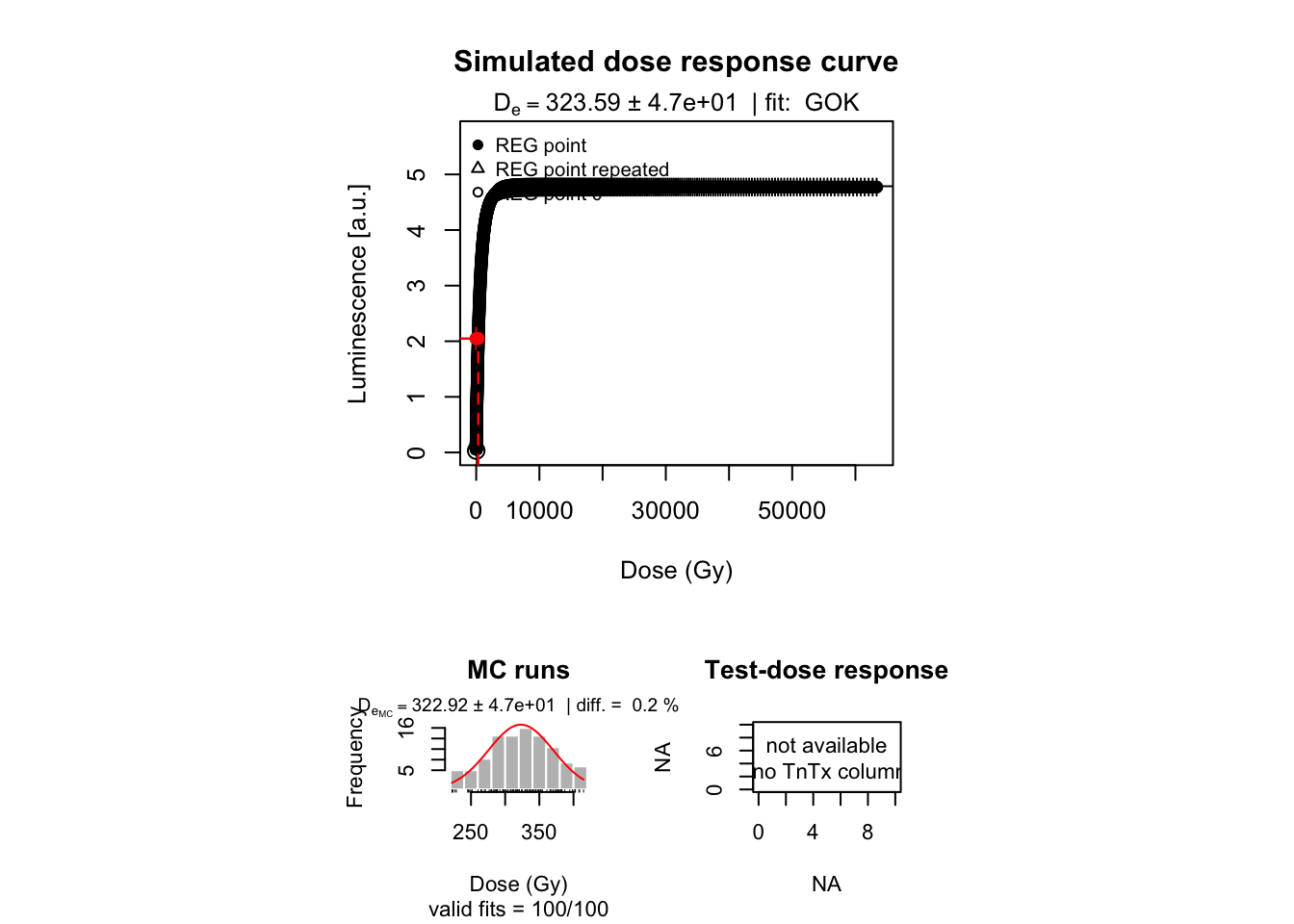
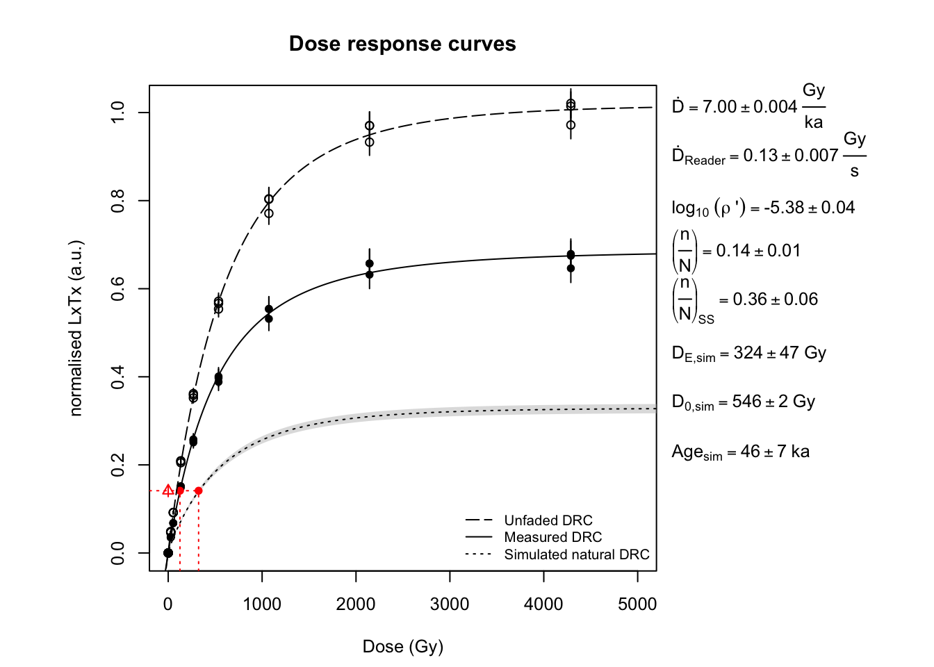
## [calc_Huntley2006()]
## 
##  -------------------------------
##  (n/N) [-]:	 0.14 ± 0.01
##  (n/N)_SS [-]:	 0.36 ± 0.06
## 
##  ---------- Measured -----------
##  DE [Gy]:	 125.14 ± 14.63
##  D0 [Gy]:	 524.75 ± 19.69
##  c [-]:		 0.33 ± 0.07
##  Age [ka]:	 17.88 ± 2.27
## 
##  ---------- Un-faded -----------
##  D0 [Gy]:	 604.45 ± 14.54
##  c [-]:		 0.2 ± 0.06
## 
##  ---------- Simulated ----------
##  DE [Gy]:	 323.59 ± 47.35
##  D0 [Gy]:	 546.44 ± 2.44
##  c [-]:		 0.26 ± 0
##  Age [ka]:	 46.23 ± 7.15
##  Age @2D0 [ka]:	 156.13 ± 7.84
##  -------------------------------

Please note that the entire function, and especially the GOK fit is a beta version, and you should verify your results carefully.

References

Huntley, D.J., 2006. An explanation of the power-law decay of luminescence. Journal of Physics: Condensed Matter 18, 1359-1365. doi:10.1088/0953-8984/18/4/020
Huntley, D.J., Lamothe, M., 2001. Ubiquity of anomalous fading in K-feldspars and the measurement and correction for it in optical dating. Canadian Journal of Earth Science 38, 1093-1106. doi: <10.1139/cjes-38-7-1093>
Kars, R.H., Wallinga, J., Cohen, K.M., 2008. A new approach towards anomalous fading correction for feldspar IRSL dating - tests on samples in field saturation. Radiation Measurements 43, 786-790. doi:10.1016/j.radmeas.2008.01.021
Sanderson, D.C.W., 1988. Fading of thermoluminescence in feldspars: Characteristics and corrections. Nuclear Tracks and Radiation Measurements 14, 155-161.
Templer, R.H., 1986. The localised transition model of anomalous fading. Radiation Protection Dosimetry 17, 493-497.
Visocekas, R., 1985. Tunnelling radiative recombination in labradorite: Its association with anomalous fading of thermoluminescence. Nuclear Tracks and Radiation Measurements 10, 521-529.
Wintle, A.G., 1973. Anomalous fading of themroluminescence in mineral samples. Nature 245, 143-144.
Wintle, A.G., 1977. Detailed study of a thermoluminescent mineral exhibiting anomalous fading. Journal of Luminescence 15, 385-393.