Give me energy: convert_Wavelength2Energy()

Since a few years ‘Luminescence’ includes functions to treat and display 3D emission spectra, e.g., plot_RLum.Data.Spectrum(). Such spectra are usually recorded on a wavelength scale but need to be transposed to energy scales, e.g., to deconvolute individual peaks by fitting. For emission spectra it needs more than just replacing the wavelength axis, but also the signal values need to be recalculated to maintain the area under the sum spectrum (example after Mooney et al., 2013).

A simplified form of such conversion was already included in plot_RLum.Data.Spectrum(), but the values could not be extracted. To quicken and unify the workflow among the package ‘Luminescence’ now convert_Wavelength2Energy() takes over and is also used internally by plot_RLum.Data.Spectrum(). Output values are similar to the allowed input values ( RLum.Data.Spectrum(), data.frame and matrix). Example:

plot(
 convert_Wavelength2Energy(xy),
 xy$y,
 type = "l",
 xlim = c(1.23, 8.3),
 xlab = "Energy [eV]",
 ylab = "Luminescence [a.u.]"
)

Life is short: fit_OSLLifeTimes()

New equipment brings new data, brings new challenges. Back in late 2017, we got our first nanosecond pulsing unit shipping to Bordeaux. The project aimed at investigating very short luminescence signal lifetimes in quartz in minerals. To analyse the data and deconvolve the bulk signal, a series of photons arriving after an OSL pulse, Sebastian and Christoph S. created a new function using ideas proposed by Bluszcz and Adamiec (2006) to identify a statistically justified number of lifetimes components.

The function works on RLum.Data.Curve, data.frame or matrix objects and runs a differential evolution algorithm to identify meaningful start parameters later piped into a nonlinear least square fitting.

fit_OSLLifeTimes(
object = ExampleData.TR_OSL, 
verbose = TRUE)

Show it all: plot_DRCSummary()

You have always been wondering how the dose-response curves would look like if combined in a single plot? Now we have a solution: plot_DRCSummary() works directly on the output of the function analyse_SAR.CWOSL() and extracts the equations with the fitting parameters for you, and it displays everything in a single plot. Of course, it also works on a list of objects created by analyse_SAR.CWOSL().

plot_DRCSummary(
  object = results,
  show_natural = TRUE,
  show_dose_points = TRUE
)

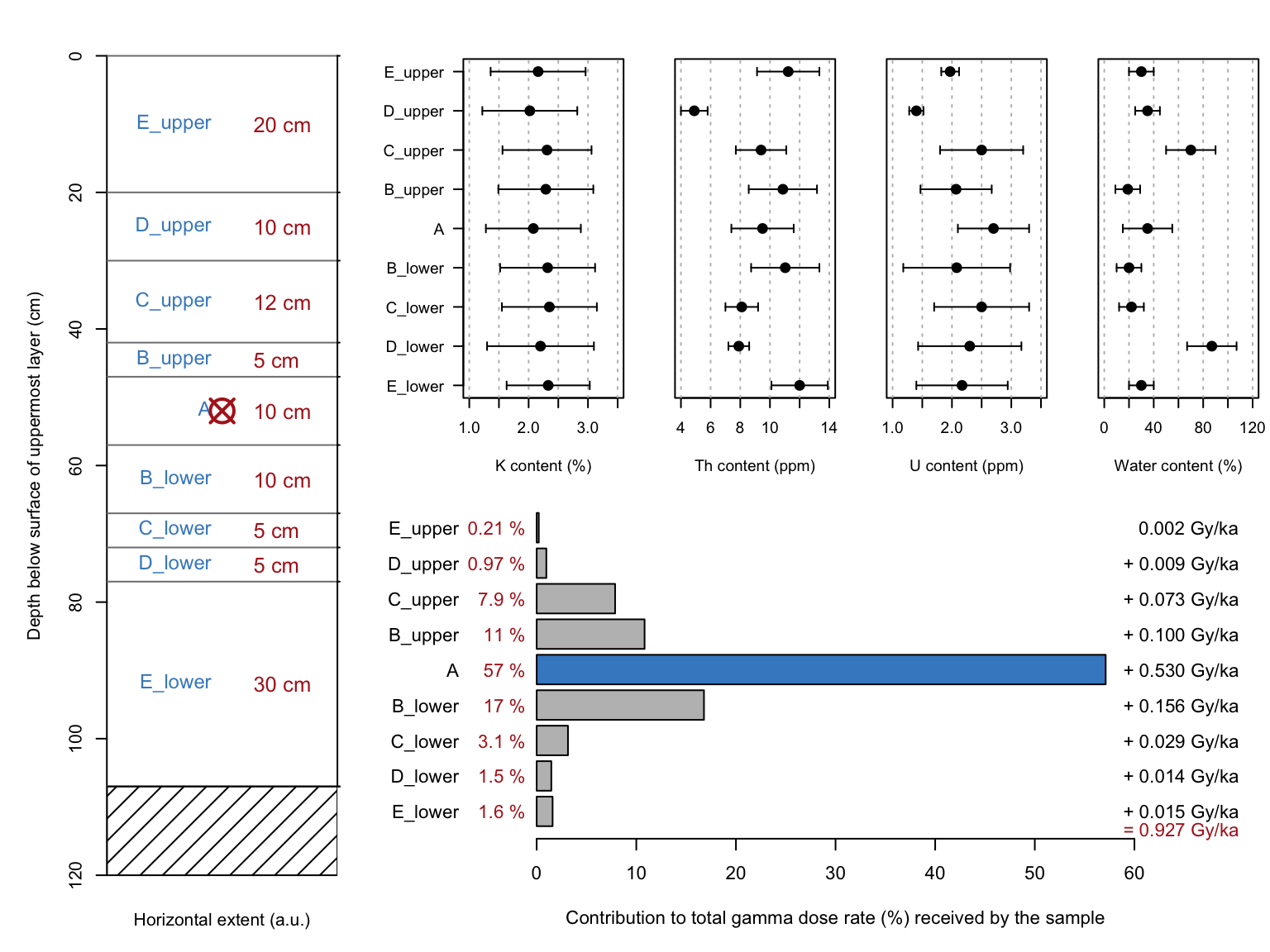
Nothing is as it seems: scale_GammaDose()

Scale the \(\gamma\)-dose rate considering layer-to-layer variations in soil radioactivity. The first contribution by S. Riedesel and M. Autzen. The range of \(\gamma\)-radiation requires corrections to be made for the dose received by a sample when situated within a complex sediment sequence. If no portable \(\gamma\)-ray spectrometry was performed, individual dosimetry samples should be taken within the influencing distance for \(\gamma\)-radiation. The function allows the user to input element concentrations for U, Th and K for all samples taken from layers that may impact the \(\gamma\)-dose received by the luminescence sample. The function calculates the \(\gamma\)-dose rate received by the samples using the superposition approach according to Aitken (1985). The user will also be provided with details on the contribution of each sediment layer to the overall dose rate and a figure showing details of the sediment sequence, element concentrations of the samples and dose rate contributions.

results <- scale_GammaDose(
  data = ExampleData.ScaleGammaDose,
  conversion_factors = "Cresswelletal2018",
  fractional_gamma_dose = "Aitken1985",
  verbose = FALSE,
  plot = TRUE
)

Completing the toolset: fit_ThermalQuenching()

Investigating thermal quenching of luminescence signals (e.g., Wintle, 1975) using pulsed-annealing experiments are one of the fundamental experiments to determine defect parameters, such as the energy depth of an electron trap. What was missing so far was a function in ‘Luminescence’ ready to be used on your datasets, fit_ThermalQuenching() closes this gap and could not be easier to be used:

fit_ThermalQuenching(
 data = data)

References

Aitken, M.J., 1985. Thermoluminescence Dating. Academic Press, Oxford.
Bluszcz, A., Adamiec, G., 2006. Application of differential evolution to fitting OSL decay curves. Radiation Measurements 41, 886–891. doi: 10.1016/j.radmeas.2006.05.016
Mooney, J., Kambhampati, P., 2013. Get the Basics Right: Jacobian Conversion of Wavelength and Energy Scales for Quantitative Analysis of Emission Spectra. J. Phys. Chem. Lett. 4, 3316–3318. doi: 10.1021/jz401508t
Wintle, A.G., 1975. Thermal Quenching of Thermoluminescence in Quartz. Geophys. J. R. astr. Soc. 41, 107–113.